Vertex Shader Domain Warping with Automatic Differentiation
A few years ago, I wrote a blog post about how to warp 3D objects in a shader and still have correct normals. It got the job done for me at the time, but the algorithm I used then wasn't quite as simple as I thought it could be, and it had a few degenerate points where it broke down. In the time since writing that, I've seen a few people talk about the problem like it couldn't be solved, so I figured maybe it was time to write up the final equations and publish it in a more referenceable package.
Background: domain warping
Creative coding is an art form that uses the computer and source code as an expressive medium. To be able to work quickly and iteratively, the techniques that get a strong foothold in the community are the ones where there are easily tweakable parameters that lead to a wide variety of outputs.
One such technique is domain warping, used often in 2D and some 3D contexts. Let's say you have a function offset(point) that defines an offset to apply to any point in space. This would be a function that takes in a vector and outputs another vector. To produce a warped point with that offset function, you would use:
function warp(point) {
  return point.add(offset(point))
}
Now, any function that would normally work on a point in space, you could instead supply with warp(point) to produce a domain-warped version. This can be as simple as just drawing a shape to the screen: instead of drawing points, lines, or curves, you could warp all of them with first, and then draw the results.
Domain warping creates a framework that invites exploration, as any offset function can be used, producing varied, interesting results from combinations of simple mathematical building blocks.
The problem: applying warps to 3D meshes
The traditional realtime 3D graphics pipeline involves creating shapes out of triangle meshes and passing them through two phases of a rendering pipeline: first, every vertex is processed in parallel to position the 3D vertices on the 2D screen, and then every pixel on the screen is processed in parallel to pick final colours given the output from the previous phase.
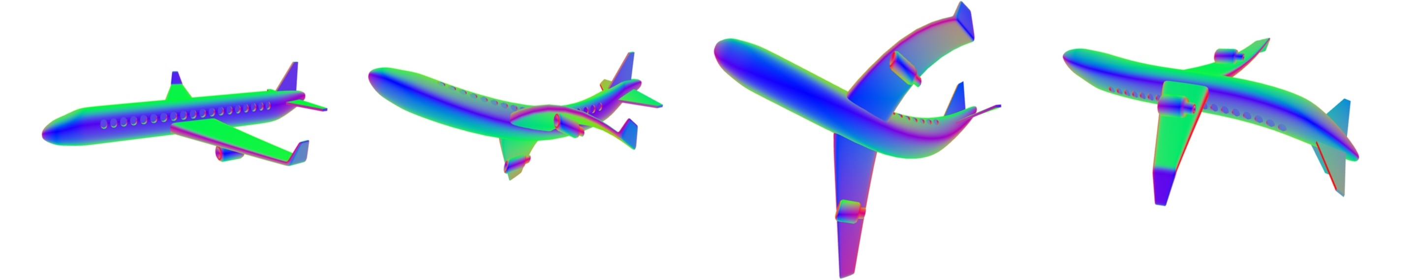
That first phase sounds like a great spot to introduce domain warping! Since we're already running on every vertex, we can apply the warp function before returning the result, and we get a very fast implementation of the warp. The trouble is that the vertex position isn't the only information being processed. We also pass in a normal, which is a vector pointing directly out of the surface of the shape. This is what you see visualized when you use normalMaterial() in p5.js.
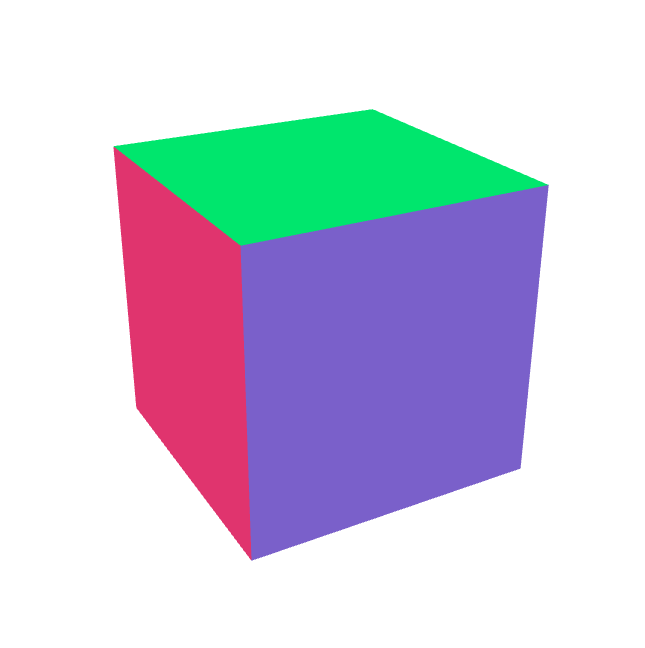
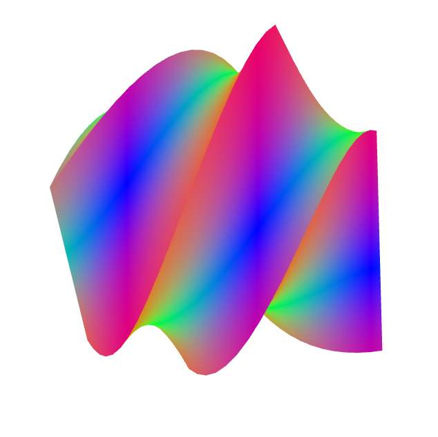
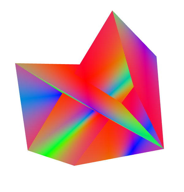
(a) Input
(b) Warp without adjusting normals
(c) Warp with screen-space derivatives
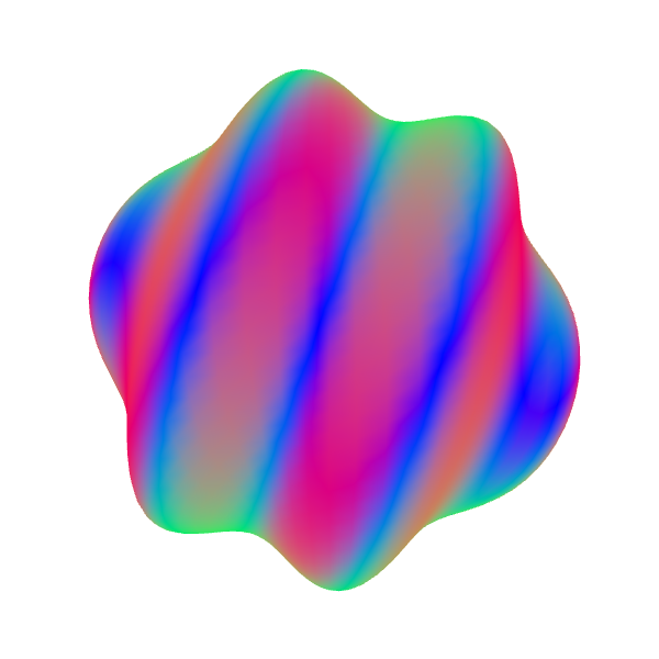
(d) Warp affecting vertices and normals
The trouble is, when you move the vertex positions around, the normals need to change in order to remain perpendicular to the warped surface. In the figure above, (b) is what you would get by just changing vertex positions, but (d) is how it should actually look. You might consider recreating the normals entirely in screen space in the fragment shader by using normalize(cross(dFdx(position), dFdy(position))), but that produces the image in (c) due to the fact that positions are only linearly interpolated across faces.
So, what can we do to get the result we want?
Fixing it with some math
We'll tackle the problem in three steps:
- Express derivatives of the warp function given a local tangent and bitangent, which we then use to generate a warped normal. Importantly, the structure of the derivative formula depends only on the warp function and accepts any local parameterization, enabling one warp shader to work on all meshes.
- Provide a formula for a surface tangent and bitangent given only the surface normal, allowing inputs to Step 1 to be generated in a vertex shader with limited knowledge of the mesh.
- Use automatic differentiation to statically generate a shader with the derivatives required for Step 1.
1. Updated normals
Let's say you have two different vectors \(\hat{u}\) and \(\hat{v}\) that are tangent to the surface of your original mesh, \(M\), at some point \(\vec{p}\). The original normal is just \(\hat{n} = \hat{u} \times \hat{v}\). On the warped mesh, one can approximate \(\hat{n}'\) by finding the result of the warp function (we'll call it \(w\)) on points near \(\vec{p}\), shifted slightly along a linear approximation of the surface by a small value \(h\):
\(\hat{n}' \approx \operatorname{normalize}\left(\frac{w(\vec{p} + h\hat{u}) - w(\vec{p})}{h} \times \frac{w(\vec{p} + h\hat{v}) - w(\vec{p})}{h}\right)\)
If you're writing a one-off shader, you can stop here and skip to step 2. You'll have to trial-and-error a good value for \(h\), but that's pretty feasible for a single shader. Inigo Quilez has some tips on that. I'm interested in making something that generalizes better, so we're going to continue on without approximations. Taking the limit as \(h \rightarrow 0\), this is equivalent to taking directional derivatives:
\(\hat{n}' = \operatorname{normalize}\left(\frac{\partial w(\vec{p})}{\partial \hat{u}} \times \frac{\partial w(\vec{p})}{\partial\hat{v}}\right)\)
We can break this down further: we know our warp function just takes the original point and adds an offset. If we call that offset function \(f\), that means \(w(\vec{x}) = \vec{x} + f(\vec{x})\):
\(\hat{n}' = \operatorname{normalize}\left(\frac{\partial (\vec{p} + f(\vec{p}))}{\partial \hat{u}} \times \frac{\partial (\vec{p} + f(\vec{p}))}{\partial\hat{v}}\right)\)
Since, by definition, \(\hat{u}\) and \(\hat{v}\) are tangent to the surface at \(\vec{p}\), the directional derivative of \(\vec{p}\) in the direction of \(\hat{u}\) or \(\hat{v}\) will be \(\hat{u}\) or \(\hat{v}\) itself, respectively:
\(\hat{n}' = \operatorname{normalize}\left(\left(\hat{u} + \frac{\partial f(\vec{p})}{\partial \hat{u}}\right) \times \left(\hat{v} + \frac{\partial f(\vec{p})}{\partial\hat{v}}\right)\right)\)
Since \(f\) is defined in terms of Cartesian coordinates and not the coordinate space defined by \(\hat{u}\) and \(\hat{v}\), we reframe the above expression to be in terms of the Jacobian of the offset, \(J=\left[\frac{\partial f(\vec{p'})}{\partial x}~\frac{\partial f(\vec{p'})}{\partial y}~\frac{\partial f(\vec{p'})}{\partial z}\right]\):
\(\hat{n}' = \operatorname{normalize}\left(\left(\hat{u} + J\hat{u}\right) \times \left(\hat{v} + J\hat{v}\right)\right)\)
To define \(J\), we calculate all the partial first-order derivatives of \(f\). Turns out, computers are great at doing derivatives, so you won't have to do them by hand, but we'll get back to that later. Importantly, this is independent of the choice of tangent vectors: whichever ones we pick, the formula for \(J\) does not change, so we do not need to run automatic differentiation at runtime. It is sufficient to run it once at compile time, and our runtime choice of tangent vectors only adds a matrix multiplication with \(J\).
2. Picking tangent vectors
Without knowledge of the rest of the mesh vertices and their connectivity, we can make assumptions about the local surface around \(\vec{p}\). The normal \(\hat{n}\) implies that there is a surface plane \(S\) passing through \(\vec{p}\) and normal to \(\hat{n}\). We can parameterize this plane into a tangent \(\hat{u}\) and bitangent \(\hat{v}\) by finding any vector \(\hat{w}\) not equal to \(\pm\hat{n}\), taking the cross product between it and \(\hat{n}\) to get one vector parallel to \(S\), and then taking the cross product between that and \(\hat{n}\) to get another, different vector parallel to \(S\):
\(\begin{aligned} \hat{w} &= \begin{cases} [0~~1~~0]^T,&\hat{n} = [\pm1~~0~~0]^T\\ [1~~0~~0]^T&\text{otherwise} \end{cases}\\ \hat{v} &= \operatorname{normalize}(\hat{v} \times \hat{n})\\ \hat{u} &= \hat{v} \times \hat{n}\end{aligned}\)
3. Automatic differentiation
The key part that makes this system nice to work with is that it lets you write just a warp function, and the derivatives used for the Jacobian earlier get automatically written for you by the system. An example warp using this system looks like this:
const twist = createWarp(
  function({ glsl, millis, position }) {
    function rotateX(pos, angle) {
      const sa = glsl.sin(angle);
      const ca = glsl.cos(angle);
      return glsl.vec3(
        pos.x(),
        pos.y().mult(ca).sub(pos.z().mult(sa)),
        pos.y().mult(sa).add(pos.z().mult(ca))
      );
    };

    const rotated = rotateX(
      position,
      position.x()
        .mult(0.02)
        .mult(millis.div(1000).sin())
    );
    return rotated.sub(position);
  }
);
It's made for JavaScript where we don't have operator overloading, so it uses an object-and-method notation similar to p5.Vector methods. You define your offset function, and then the system returns a shader for you that will apply it to both positions and normals.
The underlying autodiff system is implemented in my glsl-autodiff library, and then this is used in the p5.warp library to do the math described in steps 2 and 3.
Given the offset function \(f([x~~y~~z]^T) = [0.5\sin(0.005t + 2y)~~0~~0]^T\), it would be used to produce the following GLSL:
vec3 offset = vec3(
  sin(time * 0.005 + position.y * 2.0)
    * 0.5,
  0.0,
  0.0
);
vec3 d_offset_by_d_y = vec3(
  0.5 * cos(
    time * 0.005 + position.y * 2.0
  )) * (0.0 + (2.0 * 1.0)),
  0.0,
  0.0
);
mat3 jacobian = mat3(
  vec3(0.0),
  d_offset_by_d_y,
  vec3(0.0)
);
This then gets spliced into a standard vertex shader for you:
void main() {
  // Start from attributes
  vec3 position = aPosition;
  vec3 normal = aNormal;

  // Splice in auto-generated code.
  ${outputOffsetAndJacobian()}

  position += offset;
  vec3 w = (normal.y == 0. && normal.z == 0.)
    ? vec3(0., 1., 0.)
    : vec3(1., 0., 0.);
  vec3 v = normalize(cross(w, normal));
  vec3 u = cross(v, normal);
  normal = normalize(cross(
    u + jacobian * u,
    v + jacobian * v
  ));

  // Apply camera transforms and output
  gl_Position = uP * uVM * vec4(position, 1.);

  // Pass on to fragment shader
  vNormal = uN * normal;
}
Results
One of the first sketches I made with this was a bendy, warped airplane:
This also works with other uniform data that you might want to pass into the shader, such as the mouse coordinate, leading to this treatment of the Butter logo:
I've also used the library in a number of other sketches to get fast warps without losing lighting. A common technique for me is to add some subtle wiggles to meshes to break up their rigidity and add some whimsy.
Limitations
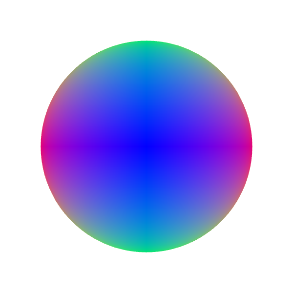
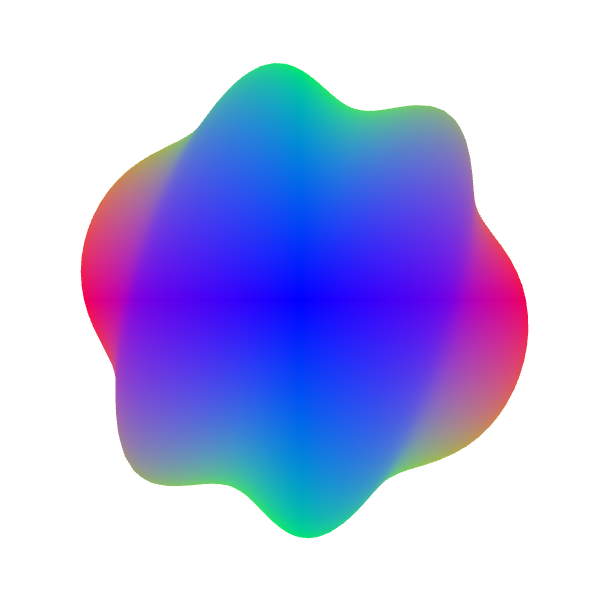
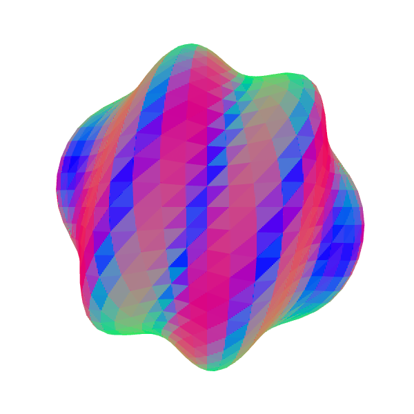
The most immediate limitation of this technique is that it can only move around existing vertices and can't create new ones. Given two points \(\vec{p}\) and \(\vec{q}\) connected by a straight edge on a mesh \(M\), the ideal form of the domain warped mesh has \(\vec{p'}=w(\vec{p})\) and \(\vec{q'}=w(\vec{q})\) connected by a curve \(C(t) = w(t\vec{p} + (1-t)\vec{q}),~t\in[0,1]\). Since the outputted mesh in WebGL will still connect \(\vec{p'}\) and \(\vec{q'}\) with the straight line segment \(L(t) = tw(\vec{p}) + (1-t)w(\vec{q})\), the visual quality of a deformed mesh depends highly on the distance between the ideal curve \(C(t)\) and its approximation \(L(t)\). OpenGL has tessellation shaders, so if you're interested in porting this to desktop and adding automatic subdivision, let me know!
(a) Input
(b) Warped, 20 edges/side
(c) Warped, one edge/side
Future work
This is a problem aimed mostly at the standard mesh-based WebGL pipeline. Already, you don't need any of this if you're raymarching signed distance fields in a fragment shader. It's entirely possible that in a few years, we'll be using custom pipelines implemented via WebGPU compute shaders which have their own limitations. At that point, we'll probably need some new math to get different creative coding techniques working, so expect some updates!